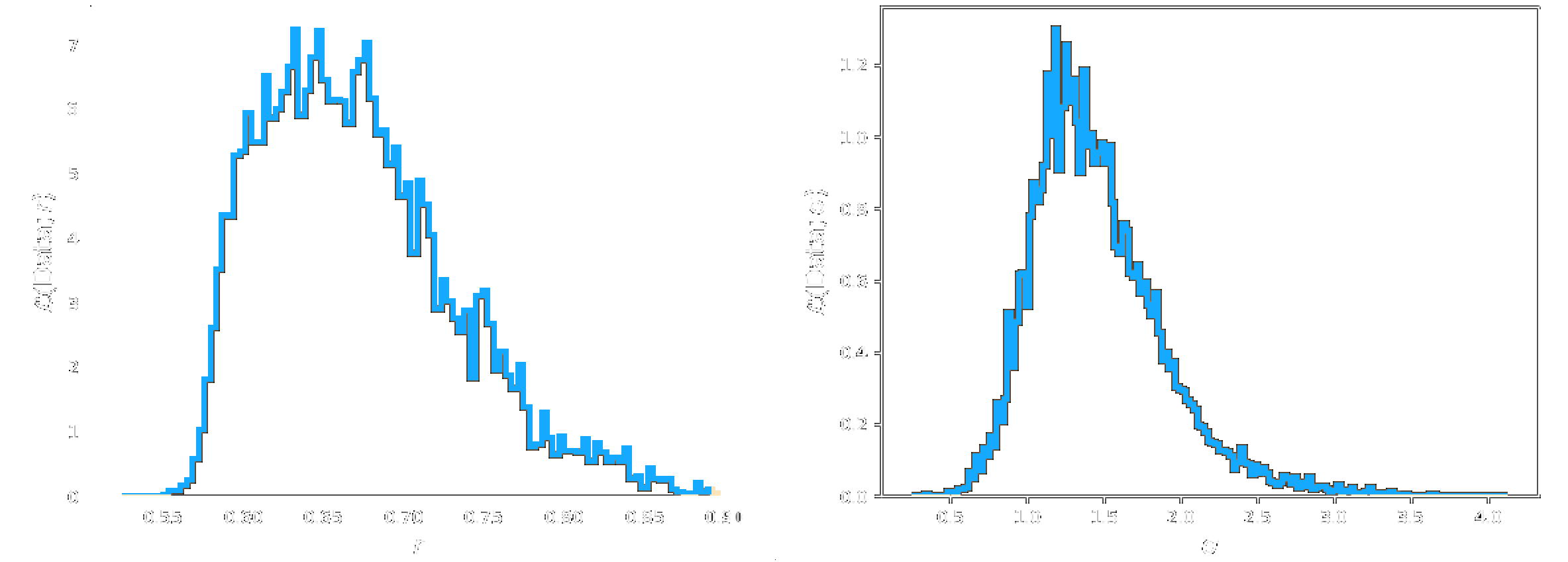
Figure 14: Marginal posteriors obtained from 10,000 iterations of MH and AM algorithms on simulated data.
We seek the posterior parameter distribution $p(\theta|D)$ where the parameter vector $\theta = [X_0,r,\alpha,\sigma]$, implementing primarily the Metropolis Hastings algorithm, and subsequently Adaptive Metropolis. Uniform priors are chosen for each of the target parameters: $$ p(X_0) = U(0,\infty), \quad p(r)=U(0,1), \quad p(\alpha)=U(0,\infty),\quad p(\sigma) = U(0,\infty). $$
Marginal Posteriors: Simulated Data
To test the MH and AM algorithms, parameter inference was performed on data simulated from known values of $X_0, r, \alpha$ and $\sigma$. The data simulated corresponds to the forward simulation of the process discussed in Model, with $X_0=50, r=0.6$. Additionally, Gaussian noise is added with zero mean and $\sigma=0$ also.
Marginal posteriors were obtained for $X0, r$ and $\sigma$. We have omitted $\alpha$ from the discussion henceforth as, in general, both algorithms exhibited poor inference for the parameter. As a matter of fact, Lalam, 2007 considers $\alpha$ as a known constant, and no method is specified to determine its value. Whilst in this project analogous methods for determining other parameters in the model were attempted, results were uninformative. It is in fact the case that variability in $\alpha$ can cause significant uncertainty in estimates of $X_0$, due to their co-dependency.
It is clear from comparison of the marginal posteriors obtained that the MH algorithm certainly infers parameters that are closer to those known for the simulated data (Figure 14). It has been found that, whilst performing well in high-dimensional systems, AM takes many iterations to 'learn' the true target covariance matrix for the transition kernel (Roberts and Rosenthal, 2009). The AM algorithm may perform better given an increased number of iterations and more time for execution, however due to time constraints and 'trial and error' required for these methods in general (see Discussion), the MH algorithm is the primary method implemented henceforth.
Figure 15: Marginal posteriors obtained from 10,000 iterations of MH on experimental data from single-cell qPCR experiment 10-3-17 well 253.
Marginal Posteriors: Experimental Data
The MH algorithm is implemented on data from single-cell qPCR experiment 10-3-17 well 253. Marginal posteriors obtained from 10,000 iterations are shown in Figure 15. Posteriors shown here are merely indicative. True interpretation of posteriors requires analysis of chain mixing (consideration of time series and autocorrelation functions), which upon further inspection reveal the Markov chain is 'cold' (see Discussion). For marginal posteriors, trace plots, and ACF figures for all model parameters from inference on qPCR data well 253 experiment 10-3-17 please click here:
To investigate the effects of increasing execution time for the algorithm, as well as considering the AM method, results for $X_0$ (the target parameter of highest importance) from MH 10,000 iterations, MH 100,000 iterations, and AM 100,000 iterations are shown for comparison in Figures 16 and 17.
Figure 16 indicates that executing the MH algorithm for longer does not in fact improve the marginal posterior distribution we obtain. However, inspecting the trace plots and ACF figures for this run of 100,000 shows an improvement in Markov chain mixing (see Full Results Figures), over all parameters except $X_0$. It appears to be the case that the Markov chain is too cold, and simply running the algorithm for an extended time period allows the chain to veer away from the true posterior distribution. One possible solution to this problem would be to impose a stricter prior upon $X_0$, for example $p(X_0)=U(0,100)$ as opposed to $U(0,\infty)$. Results from imposing this stricter prior can be found under Full Results Figures. It shows a mild improvement in the mixing of the Markov chain, however the chain is still classified as 'cold'.
Figure 17 shows that, as discussed previously, implementing the AM algorithm for an increased number of iterations appears to capture the posterior more effectively. However, this posterior is significantly dissimilar to that obtained from MH for 10,000 iterations. Moreover, inspection of the time series and autocorrelation functions is required to attain if the posterior can be interpreted appropriately. See Full Results Figures for the complete results figures for 100,000 iterations of AM. The Markov chain is, again, cold. Alterations to the transition kernel $q$ may improve chain mixing. Alternatively, performing AM for a certain number of iterations, and then freezing the covariance matrix, to then simply implement MH for the remaining number of iterations to be executed may also improve the results.
Primary adjustments that can be made to methods include increasing execution time (extending the number of iterations), and experimenting with priors. For further details of potential adjustments to implementation of methods see Discussion.
Figure 16: Marginal posteriors obtained from 10,000 and 100,000 iterations of MH on experimental data from single-cell qPCR experiment 10-3-17 well 253.
Figure 17: Marginal posteriors obtained from 100,000 iterations of MH and AM on experimental data from single-cell qPCR experiment 10-3-17 well 253.