Mitochondrial DNA

Mitochondrial DNA (mtDNA) is a closed, double-stranded DNA circle located in mitochondria, where it exists on the scale of hundreds of thousands of copies in an individual. It encodes a number of essential mitochondrial proteins, as well as molecules necessary for intramitochondrial translation. As a result of its unique maternal inheritance pattern and relatively high mutation rate, mtDNA is often used in evolutionary biology and population genetics studies.

Figure 1: Heteroplasmy as a result of replication, and the existence of a biochemical threshold. Figure adapted from Stewart and Chinnery, 2015.

Heteroplasmy

Heteroplasmy is the presence of more than one type of organellar genome within a cell or individual. Mutations that occur during replication result in heteroplasmy. It can be described by a ratio $m/(w+m)$, with $m$ denoting the number of mutant DNA molecules present, and $w$ the number of wildtype (non-mutant) molecules. In the context of this study, heteroplasmy refers to the presence of more than one form of mtDNA in a cell.

Heteroplasmy is not always harmful, however it has been shown that heteroplasmic mutations of mtDNA are an important source of human diseases. A biochemical threshold exists, such that a functional defect occurs only above a certain level of heteroplasmy (e.g. $h = m/(w+m) \geq 0.8$ results in a defect). Figure 1 shows two sources of heteroplasmy as a result of replication, and the existence of a biochemical threshold. Vegetative segregation occurs during mitotic cell divisions, and results in daughter cells that contain a random sample of the parent cell's mtDNA. Additionally, individual mtDNAs replicate at random within a cell, making one or more copies at a time while maintaining a relatively constant total number of mtDNAs (Chinnery and Samuels, 1999).

Figure 2: Structure of the human mitochondrial genome, and corresponding connections with several human diseases. This picture is adapted from work by Shanel Kalicharan.

Motivation

mtDNA mutations contribute to human disease across a range of severity. The most severe of these mutations often affect the nervous system, muscles, heart and endocrine organs, whereas mutations that have a milder effect can result in common complex traits and late-onset disorders (Stewart and Chinnery, 2015). Furthermore, similar mutational signatures have been observed across cancer types, with mtDNA copy number showing variations within and across cancers in correlation with clinical variables (Yuan et al., 2017). The ability to quantify heteroplasmy in mtDNA is therefore key in studying age-related disease, cancers, and other health issues.

Quantification can be relative or absolute. In relative quantification, genetic differences are analysed in a given sample relative to another reference sample (such as an untreated control sample). This yields a dimensionless quantity e.g. a cell posesses 3$\times$ the mtDNA copy number of another. The objective of absolute quantification is to measure quanitites that possess dimensions e.g. a cell possesses a total of 40 mtDNA molecules. Absolute quantification is essential when constructing a mathematical model that aims to describe the world at a fundamental level, as quantities in the world are dimensional. Absolute quantification is in fact a requisite for constraining such mathematical models, furthering our fundamental understanding of processes. If we can achieve fundamental understanding, we can perhaps rationally intervene e.g. reducing heteroplasmy to restore cells to a healthy state. The goal of this project is absolute quantification of mtDNA, to obtain explicit quanitites of target analytes in order to investigate heteroplasmy and its effects.

Quantitative analysis of mtDNA is challenging in both experimental and computational aspects. Single cell data by nature is concerned with small numbers of molecules. These low copy numbers result in stochasticity, adding complexity to the task of analysis. Two different approaches to quantification arise from two types of data: scRNAseq (single-cell RNA sequencing) data, and fluorescence data from qPCR (quantitative PCR).

scRNAseq data

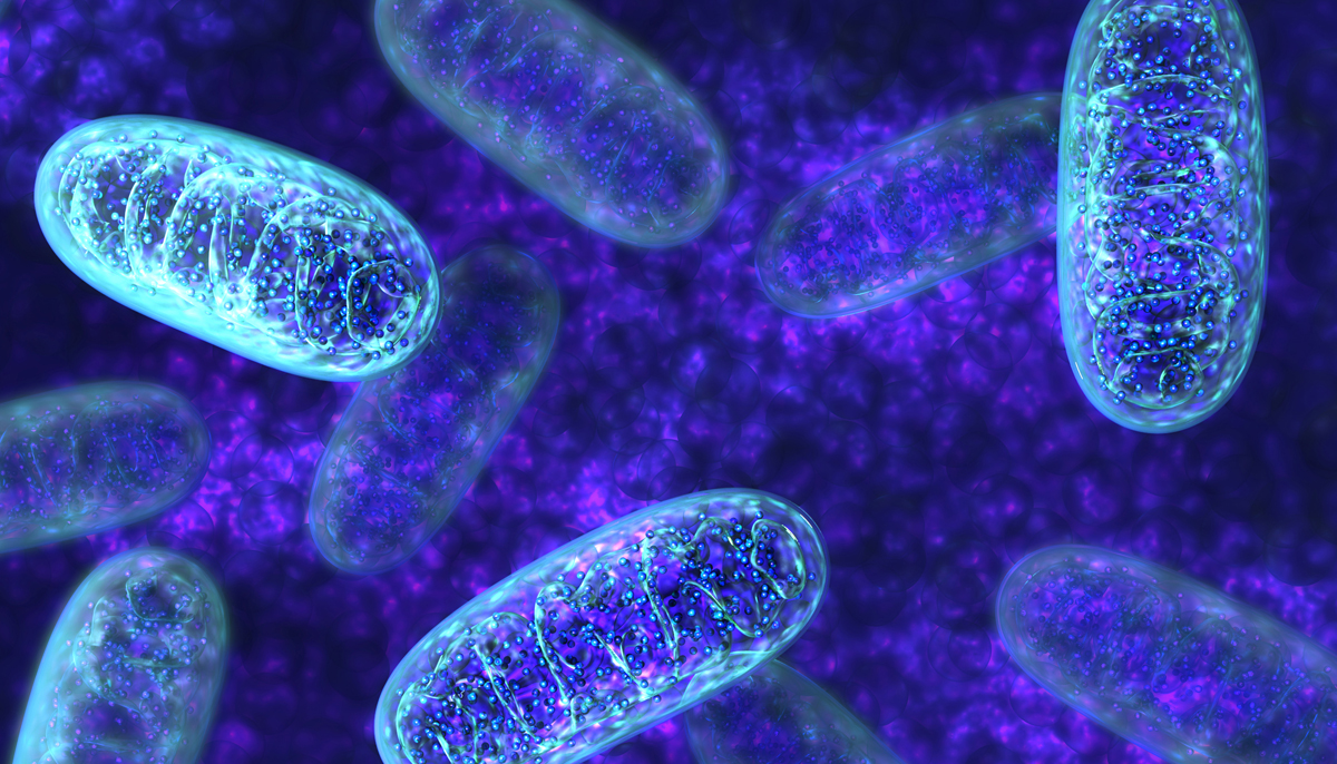
New technology (first published by Tang et al. in 2009) allows genome-wide transcriptome data to be obtained from single cells, through the use of high-throughput sequencing (scRNAseq). Across a population of cells, the distribution of expression levels for each gene are obtained. An advantage of scRNAseq over other methods (e.g. bulk RNA-seq or single-cell real-time qPCR) is the increased cellular resolution and the genome wide scope. At present there is ample scRNAseq data that has yet to be thoroughly explored in the context of absolute quantification of mtDNA. It is intuitive to consider using the transcriptome of a single cell to infer its heteroplasmy, using for instance (sparse) linear regression (Murphy, 2012). Applying techniques for analysing scRNAseq data has the potential to achieve our goal of determining mtDNA heteroplasmy, and therefore understanding how scRNAseq data is processed is key.

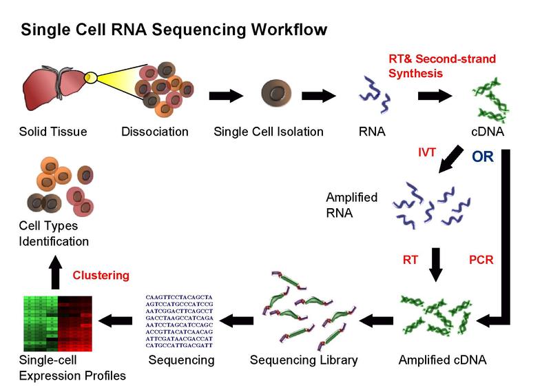
Figure 3: Single cell RNA sequencing workflow (source: Kiselev et al., 2018).

Figure 3 summarizes the overall scRNAseq workflow. RNA obtained from single cell isolation is fragmented, and cDNA is synthesized complementary to these fragments. The cDNA is amplified, forming a sequencing library. Reads are obtained after sequencing has occured. A 'read' refers to the sequence of a section of a unique fragment. A higher number of unique reads of each region of a sequence results in a higher 'sequencing depth'. Expression profiles are obtained through mapping, assigning reads to corresponding transcripts. If an RNA is expressed in high quantities, there will be more reads coming from it.

Kiselev et al., 2018 outline a scRNAseq pipeline that incorporates computational and statistical methods available. The ideal scRNAseq pipeline involves considering experimental design, processing reads, preparing the expression matrix, and interpreting biological analysis. Experimental design is important as it has implications on the biological analysis that can be carried out downstream. As each sequencing library represents a single cell, significant attention has to be paid to comparison of the results from different cells. Discrepencies are introduced due to low starting amounts of transcripts since the RNA comes from one cell only. It is possible to alleviate these issues through normalization and corrections.

A main source of discrepancy between the libraries are gene ‘dropouts’, in which a gene is observed at a moderate expression level in one cell but is not detected in another cell (Kharchenko, Silberstein, and Scadden 2014). Dropouts potentially arise because a gene was not expressed in the cell and hence there are no transcripts to sequence. However, dropouts can also be a result of experimental shortcomings: a gene was expressed but transcripts are lost prior to sequencing, or sequencing depth is not sufficient to produce any reads. One possible solution to this problem is to impute the dropouts in the expression matrix, 'filling in' the missing values and data. Two available imputation methods are MAGIC (van Dijk et al. 2017) and scImpute (Li et al. 2018). MAGIC imputes missing expression values by sharing information across similar cells, based on the idea of heat diffusion. scImpute determines which values are affected by dropout events based on a mixture model which learns each gene’s dropout probability in each cell.

The scRNAseq techniques described by Kiselev et al. can in principal be applied to mitochondria and mtDNA in order to quantify heteroplasmy. Additionally, in order to study the effects that mtDNA heteroplasmy has on nuclear DNA, transcriptomes of cells with varying heteroplasmy can be compared. 
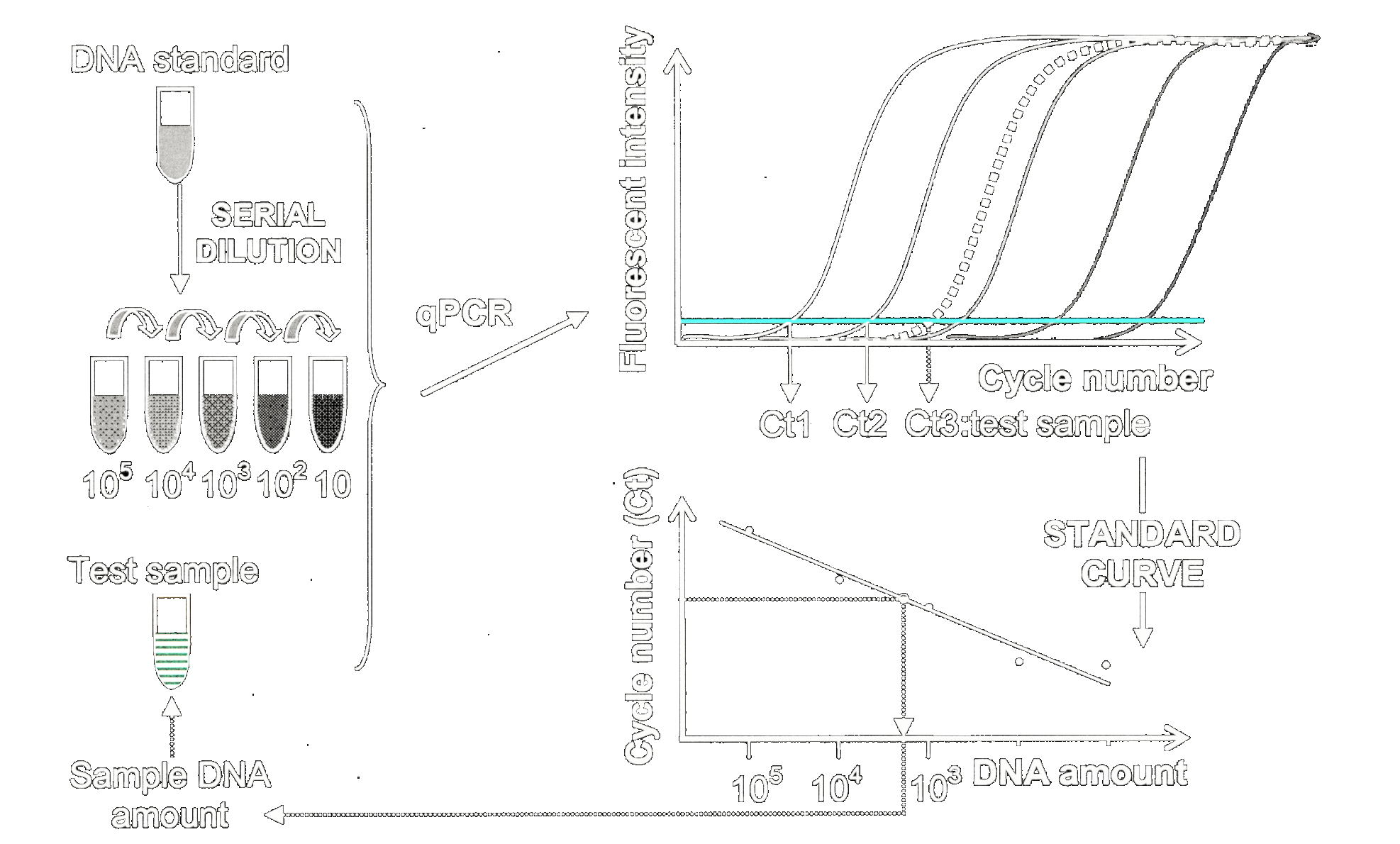
An alternative approach uses qPCR data for quantification of heteroplasmy in mtDNA, which is the main focus of this project henceforth.

qPCR data

mtDNA in single cells is present in too low a quantity to be measured and analysed directly. qPCR is an experimental technique that amplifies the quantity of a DNA segment, allowing more of the molecule to be available for experimental analysis in addition to absolute inference of copy number. It involves repeatedly heating and cooling DNA segments whilst mixing with free nucleotides. Molecule numbers are progressively amplified, and a fluorescence measurement can be obtained for each cycle. This fluorescence measurement indicates the number of molecules present at that point.

Figure 4: A simple representation of PCR. At each cycle a DNA molecule is denatured, mixed with primers (red) and free nucleotides (yellow) to form two new DNA strands. The process is 'semi-conservative', as each new DNA molecule consists of one new strand and one original strand that served as the template. After $n$ cycles, one DNA molecule yields $2^n$ replicates. This picture is adapted from work by Khan Academy.

Figure 5: Cell contents are split into two wells, such that half of the contents can be measured with qPCR detecting only mutant mtDNA, and the other half measured with qPCR detecting all mtDNA molecules.

Heteroplasmy can be quantified by partitioning mtDNA molecules obtained from a single cell into two halves, and performing qPCR on each partition. We can measure the amount of mtDNA present in one partition. In the second partition, we can measure the amount of only the mutated mtDNA present. The ratio of these measurements tells us the level of heteroplasmy.

The Standard Curve Method

The standard curve method has been used extensively in absolute quantification of parameters from qPCR data. A calibration curve from samples with known properties is constructed. For qPCR data, the standard curve method is known as the comparative $C_T$ method, also referred to as the $2^{-\Delta \Delta C_T}$ or Double Delta Ct method (Schmittgen and Livak, 2008).

For each standard in a set of samples where the initial number of molecules $X_0$ is known, the cycle number $C_T$ where the fluorescence exceeds a fixed threshold $T$ is recorded. A calibration curve is constructed from the $(X_0,C_T)$ for each standard. The set of standards is often a dilution series, where the initial copy number is progressively diluted in, for example, factors of 10. This results in a linear calibration curve when plotting $\log(X_0)$ against $C_T$.

Figure 6: Procedure for constructing of a standard (calibration) curve from a DNA standard. This picture is adapted from work by Jacquie T. Keer.

This method of constructing a calibration curve, and the standard curve method overall, has major disadvantages: it assumes the amplification efficiency is constant, and does not take into account the stochasticity of qPCR (see Model). Therefore, a more sophisticated approach is desirable for accurate estimation of $X_0$, especially in the limit of small copy numbers as is our circumstance.

Aims

The primary aim of this project is to perform inference for the model in Lalam 2007 (see Model for more detail) with qPCR data. Secondary to this primary aim is to perform inference efficiently, by exploring and experimenting with variations of inference methods (see Inference for more detail). Critical analysis of results will be performed, considering fundamental processes behind the inference algorithms employed.