Stochasticity in qPCR

The qPCR amplification process is stochastic. The process is not completely efficient - it is not the case that each mtDNA molecule is duplicated per cycle. At each cycle, a molecule is successfully duplicated with a certain probability, called the reaction efficiency, denoted by $r$ (see Figure 7). A binomial branching process describes the progression of amplification, and a relationship exists between the number of molecules present and the fluorescence measurement, giving rise to a Hidden Markov Model (HMM).

Figure 7: qPCR amplification is modelled as a binomial branching process. At each qPCR cycle, a molecule is amplified with probability $r$. If $r=1$ every molecule is successfully duplicated at each cycle. If $r=0.5$, duplication success is analogous to a 'coin flip'.

Figure 8: A binomial branching process describes the hidden Markov model for qPCR. The $X_i$ are the number of molecules after each round of qPCR and are 'hidden' states. The $F_i$ are the fluorescence reads and are 'observed' states. Parameters to be inferred are highlighted in red.

Hidden Markov Model

Given fluorescence data from a qPCR experiment, the main target analyte we wish to infer is the initial mtDNA copy number $X_0$. Other model parameters may be inferred as a by-product of performing inference on $X_0$.

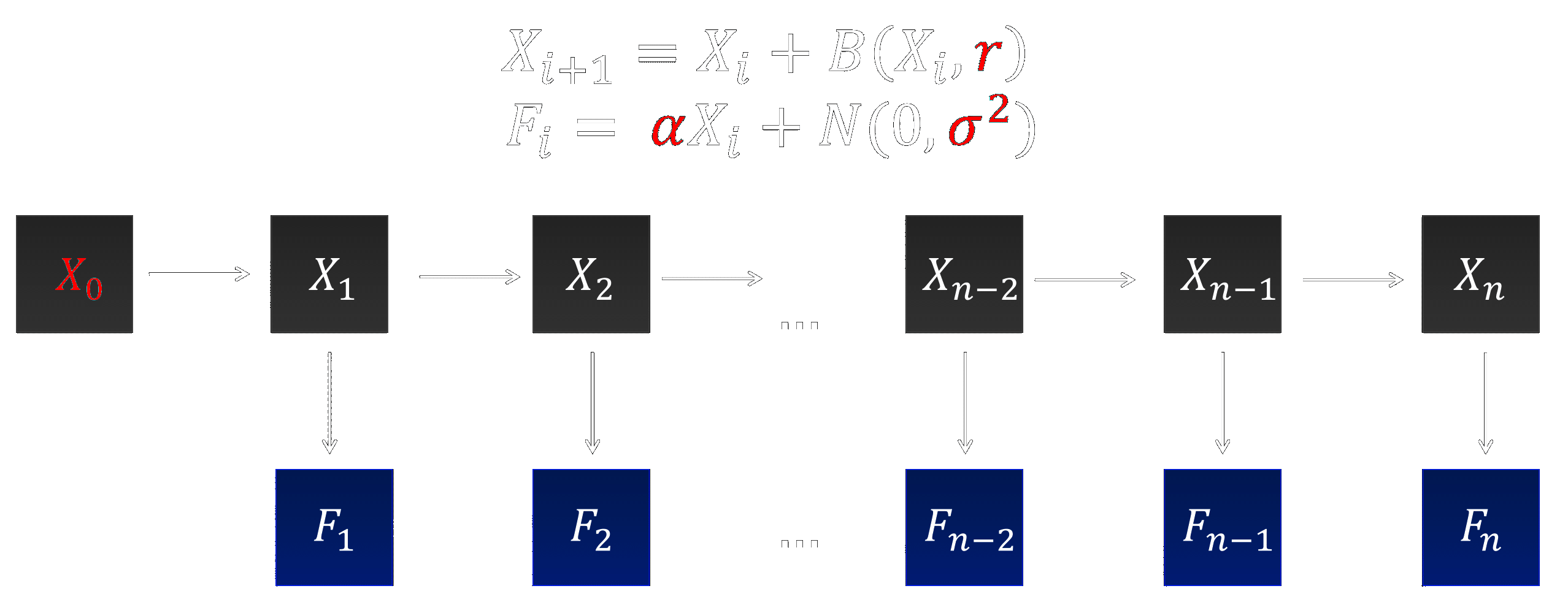
Lalam, 2007 proposes a binomial branching process combined with a HMM (Figure 8). It accounts for the fact that the number of replicated DNA molecules during qPCR is random, and additionally that the measurement of the fluorescence emitted by the DNA molecules is collected with some random error.

For all $i\geq1$: $$X_{i+1} = X_i + B(X_i,r), \qquad F_i = \alpha X_i + N(0,\sigma^2)$$ where $X_i$ is the number of molecules and $F_i$ is the measured fluorescence at cycle $i$. Fluorescence reads are taken in the presence of background fluorescence, modelled as additive Gaussian noise with mean $0$ and variance $\sigma^2$. If the experimental data used for inference is not background corrected, a different mean and variance is required.

Parameters we wish to infer are:

  • $X_0$: the initial number of molecules
  • $r$: the efficiency of the qPCR experiment
  • $\alpha$: the constant describing the proportionality of the fluorescence intensity emitted at a given cycle to the number of molecules at that point
  • $\sigma$: the variance contributing to the noise term in the fluorescence expression

Figure 9: Forward simulation of the binomial branching process, from an initial copy
number $X_0=50$, efficiency $r=0.6$. The mean and 5-95% confidence interval are
calculated from 1000 simulations of the model.

Forward Simulation

We can implement the above model to visualise the exponential amplification of the molecules, and gain intuition for the system. Due to stochasticity, a family of curves can be created for one single initial state (a fixed $X_0$, $r$). Additionally, in particular for a short amplification curve, a similar curve can be obtained by increasing the efficiency $r$ and decreasing the quantity of $X_0$. This effect induces uncertainty when performing inference on $X_0$, and other model parameters. This uncertainty can be reduced with an increased amount of data from the exponential phase of the amplification process (see Exponential Phase Identification below).

Repeatedly simulating an initial condition generates a family of curves and allows us to obtain a confidence interval for a particular combination of $X_0$ and $r$ (Figure 9).

Figure 10: A heatmap of the coefficient of variation of 1000 simulations of the qPCR process, calculated at the final cycle (cycle 30).

The smaller the efficiency $r$, the wider this confidence interval is, meaning there is less certainty of the number of molecules present after a number of cycles. Certainty decreases with each round of qPCR. This can be demonstrated by calculating the coefficient of variation at the final cycle between simulations for varying $X_0$ and $r$ (see Figure 10). For mean $\mu$ and standard deviation $\sigma$, the coefficient of variation is given by $\frac{\sigma}{\mu}$.

Limits for $r$ and $X_0$ in Figure 10 are chosen to be relevant specifically to the data analysed in this project, and have been informed by posteriors obtained through inference, which can be found in Results.

Exponential Phase Identification

qPCR data is in the form of fluorescence reads, which reach a saturation point, and also have a detection threshold. Therefore we need to discard linear and plateau phases in order for inference with binomial branching model to be successful.

To identify the exponential phase, two models – a sigmoid curve and an exponential curve – are fitted iteratively. The endmost cycle is progressively discarded from the data until the exponential curve fits ‘better’. Akaike Information Criterion (AIC) is used to determine this ‘better’ fit. The AIC measure considers both number of parameters in the model (an exponential curve uses three parameters, a sigmoid curve four) and the likelihood of the data given the model. For $k$ the number of parameters in a model, and $\hat{L}$ the maximum of the likelihood function for the model $$\text{AIC} = 2k – 2\ln(\hat{L}).$$ For the fluorescence data from single-cell qPCR experiment 10-3-17 well 253, the AIC for the exponential model is smaller at cycle 35. Therefore, the first 35 cycles correspond to the exponential phase, and these are used for inference.

Figure 11: The exponential phase is identified by using AIC model selection to determine how many cycles need to be discarded from the end prior top inference.