Bayesian Inference
One family of approaches to obtaining the posterior is the class of Markov chain Monte Carlo (MCMC) methods, which construct a Markov chain in order to sample from a probability distribution i.e. the posterior (see Figure 12). The Metropolis Hastings algorithm belongs to this family, and is classified as a random walk Monte Carlo method. This is the algorithm implemented in this project to obtain the posterior and infer target parameters.
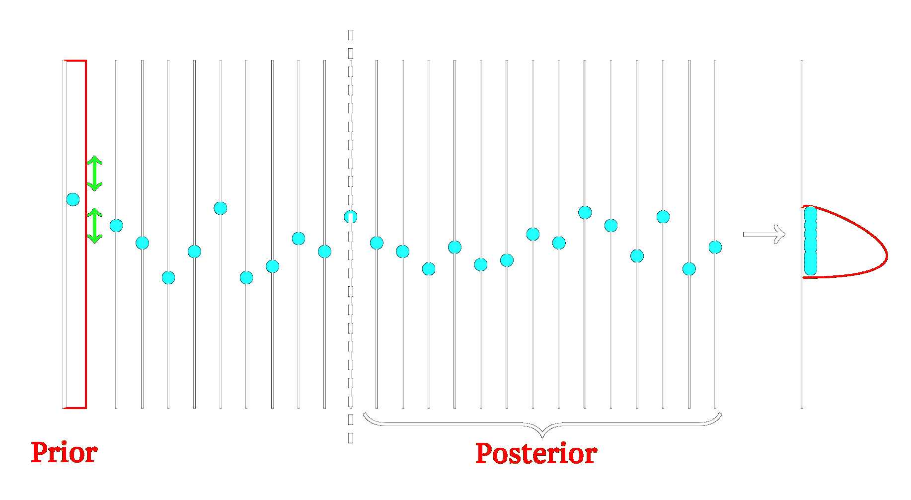
Figure 12: Visual representation of Markov chain Monte Carlo (MCMC). We can impose a prior on the parameter to aid inference. In the above example, the Markov chain is run for 10 iterations, until stationarity. All subsequent samples are from the stationary distribution, which is the desired posterior. This picture is adapted from work by MPH Stumpf.
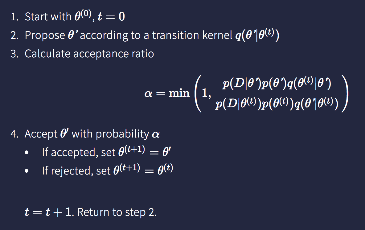
Figure 13: Metropolis Hastings Algorithm.
Metropolis Hastings Algorithm
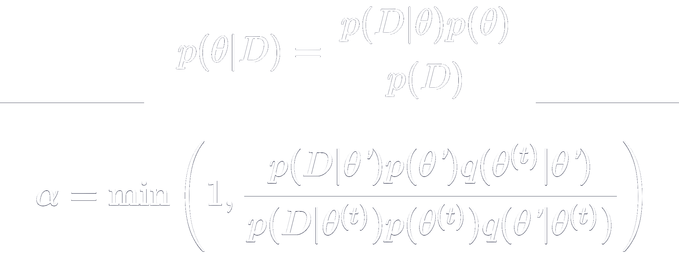
Primarily introduced in 1953 (Metropolis et al.) the Metropolis Hastings (MH) algorithm is a MCMC method for obtaining a sequence of random samples from a probability distribution for which direct sampling is difficult. A Markov chain is established and run until stationarity. All subsequent samples are from the stationary distribution, which is the desired posterior distribution.
At each iteration, the algorithm generates a candidate for the next sample value based on the current sample value. With probability $\alpha$ (the acceptance ratio), the candidate is either accepted (in which case the candidate value is used in the next iteration) or rejected (in which case the candidate value is discarded, and current value is reused in the next iteration).
Adaptive Metropolis Hastings
To experiment in increasing the computational efficiency and improving the results from the MH algorithm, we can choose the transition kernel $q$ such that this adapts according to samples from the posterior that have been accepted. The Adaptive Metropolis (AM) algorithm updates the transition kernel such that it acquires the shape of the posterior based on samples that have been accepted, allowing perturbations $\theta’$ to follow the same distribution and in theory be better at capturing the posterior as a whole (Haario et al.).
Given a 'burn-in' period of running the MH algorithm (e.g. for 10% of the total number of iterations to be carried out), the AM method computes a covariance matrix from the accepted samples from the posterior, and acquires this as the transition kernel (proposal distribution). With each additional iteration, this covariance matrix is updated based on the sample that was accepted immediately before. Due to the adaptive nature of the process, the AM algorithm is not Markovian. However, it still possesses the desired randomness we seek for our inference algorithm, and may in fact improve convergence to the posterior.